
The first part of this series took a look at the GS match rating model. The post described, how you are able to identify a non-linear relationship between the predictor variables and the outcome variable. The same methods will now be applied to the PPG match rating model, so that we are able to compare the two different polynomial regression models. On top, I want to show, how you are able to figure out, whether outliers in your data have an influence on your regression model.
Historic percentage distribution
As the GS match rating model, the PPG match rating model only consists of one predictor variable and 3 outcome variables. So we can use the same one-vs-rest approach as for the GS match rating model. At first the historic percentage distribution for each possible match outcome has to be determined:
GitHub – PPG match rating historic percentage distribution
Loading the data into RStudio works the known way:
#connect to Exasol
con <- dbConnect("exa", exahost = "[IP-adress]", uid = "sys", pwd = "exasol", schema = "betting_dv")

#load train data
train_data <- exa.readData(con, "[SQL-Query]")
The correlation test is the first starting point to compare the GS and PPG match rating.
cor(train_data$GS_MATCH_RATING,train_data$HOME_WIN_PERC)
cor(train_data$GS_MATCH_RATING,train_data$DRAW_PERC)
cor(train_data$GS_MATCH_RATING,train_data$AWAY_WIN_PERC)
The correlation test for the PPG match rating returns similar results as for the GS match rating:
Home win percentage: 0.85
Draw percentage: 0.08
Away win percentage: -0.79
Both match ratings have a strong linear relationship with the home & away win percentage. The PPG match does also not have a linear relationship with the draw percentage. But this is not surprising. The posts before already showed, that you need to use a polynomial regression to describe this outcome variable.
Linear & polynomial regression
If you did read the previous post, you should already know, how it is possible to create a simple linear regression and how to create polynomial regression model. The lm() function creates the regression model. The poly() function is used to build a polynomial of the PPG match rating variable.
#linear regression
regr_home = lm(HOME_WIN_PERC ~ PPG_MATCH_RATING, data=train_data)
regr_draw = lm(DRAW_PERC ~ PPG_MATCH_RATING, data=train_data)
regr_away = lm(AWAY_WIN_PERC ~ PPG_MATCH_RATING, data=train_data)

#summary of linear regression
summary(regr_home)
summary(regr_draw)
summary(regr_away)

#polynomial regression
poly_regr_home = lm(HOME_WIN_PERC ~ poly(PPG_MATCH_RATING,2), data=train_data)
poly_regr_draw = lm(DRAW_PERC ~ poly(PPG_MATCH_RATING,2), data=train_data)
poly_regr_away = lm(AWAY_WIN_PERC ~ poly(PPG_MATCH_RATING,2), data=train_data)

#summary of polynomial regression
summary(poly_regr_home)
summary(poly_regr_draw)
summary(poly_regr_away)
The R-squared measures for the linear regression models represent exactly the results of the regression tests. The PPG match rating correlates better with the home win percentage. That’s why, the R-squared of the home regression model is better in comparison to the GS match rating model. In comparison, the away regression R-squared is slightly worse. Surprisingly the R-squared for the linear draw model looks way better.
Linear R-squared measures:
- Regr home: 74% (53% GS)
- Regr draw: 22,5% (0,1% GS)
- Regr away: 62,5% (69% GS)
The polynomial regression models look even better. All polynomial PPG match rating models show an equal or better R-squared measure.
Polynomial R-squared measures:
- Regr home: 74% (53% GS)
- Regr draw: 37% (4,2% GS)
- Regr away: 69% (70% GS)
These were all the optimisation steps, which were already discussed in the first part.

Handling outliers
Another important step to optimise a model is the detection and treatment of outliers. Outliers are some kind of “extreme observations”, which seem not to fit or are located far away from the rest of the data. These observations need to be handled, as they may have an influence on the predicted regression model.
Following picture shows an example regression model, which is hugely influenced by a group of outliers:

Of course, this example is bit extreme. But it clearly shows, how big the difference of a regression model with and without outliers can be.
There are several methods to detect and handle outliers. I used the Cooks distance to identify the outliers. This measures identifies the impact of every prediction variable value on the regression model. The higher the influence is, the more likely is it, that this value is an outlier, which should be handled. I used 2 times the mean as the boundary for the identification.
cooksd 2*mean(cooksd, na.rm=T),names(cooksd),""), col="red") # add labels
The Cooks distance identified 6 values as outliers. These values are at the lower and upper end of our data frame. So these are the data rows with very low or very high PPG match rating. All other values have a relative similar influence on the regression model.

The diagnostic plot Residuals vs. Fitted confirms this. At the left and the right of the plot are residuals, which “stand out”. The majority of the residuals, especially in the middle, is located closer to the 0 line. This difference also indicates, that a very high and a very low PPG match rating can be interpreted as outliers.
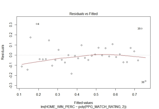
- Residuals vs Fitted diagnostic plot for PPG home regression
If we take a look at the PPG distribution, you are able to figure out, why the outliers only occur at the upper and lower bound. During a season happen only just a few games with a clear favourite. These games have either a very high or a very low PPG match rating. Because of the low number of occurrences, the historical distribution is largely influenced by the law of small numbers. Small samples need not represent the real percentage distribution and therefore can result in outliers.

- PPG match rating distribution – Bundesliga 2011-2017
So, how could you handle such outliers? There are several possibilities. You could impute mean or median data or predict the values. I tried to just ignore them. So I builded a 3rd group of polynomial regression models without outliers. Therefor, as you can identify different outliers for each regression model, you have to create 3 new data frames, which only contains the non-outliers for each regression.
#delete outlier rows
train_data_wo_o_home <- train_data[c(-1,-2,-3,-4,-35,-36), ]
train_data_wo_o_draw <- train_data[c(-3,-32,-34), ]
train_data_wo_o_away <- train_data[c(-1,-2,-3,-35,-36), ]

#polynomial regression
poly_regr_home_wo_outl = lm(HOME_WIN_PERC ~ poly(PPG_MATCH_RATING,2), data=train_data_wo_o_home)
poly_regr_draw_wo_outl = lm(DRAW_PERC ~ poly(PPG_MATCH_RATING,2), data=train_data_wo_o_draw)
poly_regr_away_wo_outl = lm(AWAY_WIN_PERC ~ poly(PPG_MATCH_RATING,2), data=train_data_wo_o_away)
Comparing the two regression lines for the away win percentage clearly shows the effect of the outliers. The last data point at the right was interpreted as an ourlier. That’s why the new regression line is not upturning for high PPG match ratings.

The R-squared measures of the new regression models now look really good. Even the draw regression model now has a value greater 50%. So you could come to the conclusion, that these models are well suited to predict the outcome of a match.
Polynomial R-squared measures without outliers:
- Regr home: 86% (74% with outliers)
- Regr draw: 63% (37% with outliers)
- Regr away: 76% (69% with outliers)
This must of course be confirmed by a comparison to the odds of the Bookies and my Poisson prediction model. The last part of this series will compare the different regression models of the GS & PPG match rating and how they perform.
The complete R code example can be found under following link:
GitHub – PPG match rating optimisation
If you have further questions, feel free to leave a comment or contact me @Mo_Nbg.
References:
[1] Ranjit Kumar Paul, Some methods of detection of outliers in linear regression models, 2014
[2] Selva Prabhakaran, http://www.r-bloggers.com/outlier-detection-and-treatment-with-r/

One Reply to “”