
The first and the second part of this series explained some basic methods to optimise the regression models for the GS & PPG match rating. You have now a set of 3 different regression models (linear, polynomial and polynomial without outliers) for each predictive variable. These models now have to not only compete against each other, but also of course against the Bookie odds and the Poisson prediction model.
Odds prediction
Before you are able to measure the performance of the models, you have to predict the probabilities and odds of the possible outcomes for matches in the past. I usually use the last 5 completed seasons and the current season as a general rule. The further back in time you want to do a prediction, the more data you need. If you use the last 5 years to build the regression model and want to predict the odds since the season 2012/13, 10 years of data have to be available.
The rating feature satellite already contains the GS & PPG match ratings needed for such a prediction. You just need to loop throw every season and predict the probabilities for each match. The easiest way would be to build the regression models based on past season and predict a full season. I have chosen a bit more complicated, but also more flexible way. For some analyses I created a new link and satellite table, which calculate the league standings for every date. The SQL code can also be found at GitHub:
GitHub – Division table satellite
These tables can be used to query each matchday and the period of time for each matchday:
matchday_data <- exa.readData(con, "
select
	division,
	season,
	played + 1 matchday,
	min(match_date) matchday_start,
	max(match_date) matchday_end
from
	(
	select
		division.division,
		season.season,
		table_l.match_date,
		min(table_s.played) played
	from
		betting_dv.FOOTBALL_DIVISION_TABLE_L table_l
		join betting_dv.FOOTBALL_DIVISION_TABLE_L_S	table_s
			on table_l.FOOTBALL_DIVISION_TABLE_LID = table_s.FOOTBALL_DIVISION_TABLE_LID
		join betting_dv.football_division_h division
			on table_l.football_division_hid = division.football_division_hid
		join betting_dv.football_season_h season
			on table_l.football_season_hid = season.football_season_hid
	where
		division.division = 'D1' and
		season.season >= '2012_2013'
	group by
		division.division,
		season.season,
		table_l.match_date
	)
group by
	division,
	season,
	played
order by
	1,2,3
")
This offers the possibility to loop throw each matchday and exactly control, when you want to re-build or re-train your model during a season. So your model will adapt to changes during a season.
Following code example shows the basic structure and processing steps for such a loop. The example just contains the loop and the processing comments. I like to use such outputs, so that I am always aware about the current step during the processing as predicting the probabilities for several seasons may take a while. This structure can be reused for every predictive model, where you have to build and train a model (e.g. Regression, Random Forest, SVM, Neural Network).
for (row in 1:nrow(matchday_data)) {
	season <- matchday_data[row, "SEASON"]
	matchday <- matchday_data[row, "MATCHDAY"]

	print(paste("Running season", season, ", matchday", matchday))

	if(matchday %in% c(1,5,10,15,20,25,30)) {
		print(paste("-Rebuilding models at matchday", matchday))

		print("--Loading train data")

		print("--Building linear regression")

		print("--Building polynomial regression")

		print("--Detecting outliers")

		print("--Building polynomial regression wo. outliers")

	}

	print(paste("-Predicting probabilities for matchday", matchday))

	print("--Loading prediction data")

	print("--Predict linear regression")

	print("--Predict polynomial regression")

	print("--Predict polynomial regression wo outliers")

	print("--Correct probabilities")

	print("--Write predicted probs to sandbox")

	#for first prediction target table has to be created
	if (row == 1) {

	} else {

	}

}
All the listed processing steps for the GS & PPG match rating models were already discussed in part 1 and part 2 of this series. You just have to combine the different steps to one single big script. As mentioned you have to train 3 types of regression models. The linear and the polynomial can directly be built with help of the training data. Before you can build the polynomial regression without outliers, you first have to identify this outliers and clean the specific train dataset.
#calculate cooks distance
gs.cooksd_home <- cooks.distance(gs.poly_regr_home)
gs.cooksd_draw <- cooks.distance(gs.poly_regr_draw)
gs.cooksd_away <- cooks.distance(gs.poly_regr_away)

#build data frames without outliers
gs.train_data.woo_home <- gs.train_data[-as.numeric(names(gs.cooksd_home[(gs.cooksd_home>2*mean(gs.cooksd_home, na.rm=T))])),]
gs.train_data.woo_draw <- gs.train_data[-as.numeric(names(gs.cooksd_draw[(gs.cooksd_draw>2*mean(gs.cooksd_draw, na.rm=T))])),]
gs.train_data.woo_away <- gs.train_data[-as.numeric(names(gs.cooksd_away[(gs.cooksd_away>2*mean(gs.cooksd_away, na.rm=T))])),]
The complete code example for the probabilities prediction can be found at GitHub:
GitHub – GS & PPG probability prediction
Model accuracy
To compare different predictive models, you have to calculate the accuracy of the predictions. I used a simple geometric mean score, to identify the best model. As this is not a build-in database function, I created a user-defined aggregate function:
GitHub – Geometric mean aggregate function
This one can than be used to query the predicted probabilities, match outcomes and calculate the model accuracy.
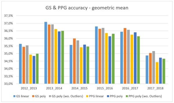
At first I took a look at the accuracy of the different GS & PPG match rating models. There are some interesting findings in that comparison.
(1) Goal difference is the better prediction variable
In the past 5 seasons and the current season every PPG match rating model has got a lower accuracy as every GS match rating model. So teams, which are positioned higher or lower in the league table compared to the goal difference of the neighbouring teams, should not be the norm. Even if a team in short-term is able to gain a positive points average with a bad goal difference, in long-term you should score more than you concede.
(2) Correlation & R-squared not always indicate a good model
The PPG match rating provides a similar correlation as the GS match rating. The R-squared of the different models was at least as high or even higher. This should have indicate, that the PPG match rating is more suited predict the outcome of the probabilities. But this is not the case. The same applies to the different GS match rating models. As the optimised models provided a higher R-squared, you would expect to be more accurate. But surprisingly the simple GS linear regression model on average provides the same accuracy.
For the comparison with the bookie and the Poisson model I just used the GS match rating. Because of the good results of the linear regression model, I builded a combined GS match rating model. The linear regression is used to determine the home and away win probability. The polynomial regression is just used for the draw probability, as there is no linear relation between draws and the GS match rating. Based on this comparison, there are some new conclusions you can draw:
(1) The Bookie is the best!
That comes at no surprise. Of course I expected the Bookie to be the most accurate in predicting the probabilities. And I did also expect to be the GS match rating model to be the worst as it is really a simple model. Interesting is the season 2016/17. The GS match rating models nearly reached the accuracy of Bet365. It will be interesting to see the influence to the Bookie simulation.
(2) The Bookie also struggles in the current season
Not only the Poisson model, also the Bookie got some problems to predict the current season of the Bundesliga. The accuracy of all models drastically decreases in comparison to the previous seasons. But also the accuracy of the Bookie is the worst in the last 6 years.
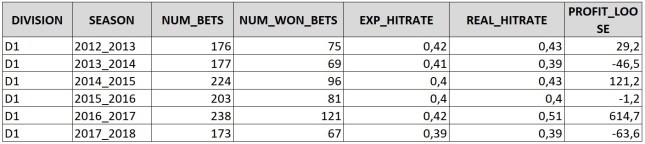
(3) Geometric mean does not indicate whether a model gains profit
Using the geometric mean score as an accuracy method, does not deliver any information about the profitability of a model. The Poisson model has always a lower accuracy, but gained profit during the seasons 2012 – 2016. The geometric mean does only respect the Back-markets (home-win, draw, away-win). But during my simulations I also identify bets for the Lay-markets (no home-win, no draw, no away-win), which have no influence on the geometric mean score.

Kicktipp simulation
By now I really like to test some new Kicktipp strategies. Kicktipp is really a huge thing in Germany. It appears as nearly every company or group of friends has a Kicktipp group. And there is also the possibility to win some money. So I also tested two Kicktipp strategies based on the GS combined model.
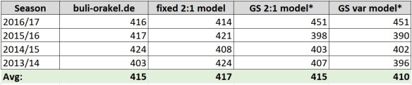
(1) GS fixed 2:1 model
This model simply picks a 2:1 win for the favoured team. This is just a modification of the fixed 2:1 model. Instead of the Bookie probabilities, I used the probabilites of the GS match rating model. The team with the higher probability to win a match is chosen as the favourite. As the outcome is always choosen a 2:1 win, as this is the result, which occurs statistically the most.
(2) GS variable model
The GS variable model also uses the probabilities of the GS match rating model to identify the possible winner of a match. But instead just picking a fixed outcome, the average number of goals scored by each team is used to guess the exact result.
The SQL code for both models can be found at GitHub:
GitHub – GS match rating Kicktipp simulation
The Kicktipp simulation reflects exactly the model accuracies. In general both models perform not as good as the reference models, except for the season 2016/17. This result is very surprising!! Both models achieved 451 points, which is the highest value of every simulation I did. The combined GS regression model reached nearly the accuracy of the Bookie during this season. And this is also represented by the Kicktipp simulation. But of course, you should keep in mind, that this certainly happened by pure chance. The other years both models fluctuate around 400 points, which is not so bad, but also not enough to win a single season.
Bookie simulation
Everything I did until now was interesting. But the main goal of building a predictive model for football matches is to test it against the odds of the Bookie. As for the Poisson model, I simulated the predicted odds against Bet365. Over- or underestimated bets should be determined for all back- and lay markets. So I had to calculate the odds for the lay markets based on the probabilities of the corresponding back market and the Bookie margin for the specific match. Overall the model simulation for the GS match rating model has 3 different parameters, which can be adapted to achieve different results. Obviously the value of a possible bet and the minimum probability for an outcome are two of them, as I already used them during the Poisson model simulation. I picked 0.2 for both parameters. Some tests showed the best results with this selection. The 3rd parameter is the range of GS match ratings, which should be used for the simulation. If you go a step back and take a look at the GS match rating distribution in one of my previous posts, you can see, that the higher and lower a GS match rating is, the lower is number of games with such a rating. So the law of the small numbers could eat up your bank. That’s why I have chosen to simulate the model with different ranges of GS match ratings and the difference in results was immense. The simulation with all matches showed a continues loss. The more I limited the match rating, the more increased the overall profit. A limit of -6 and 14 was the turning point. After that, the profit decreased again. This could be the case, as you of course also limit the number of possible matches more and more. But I was really surprised, that there was a profit at all.
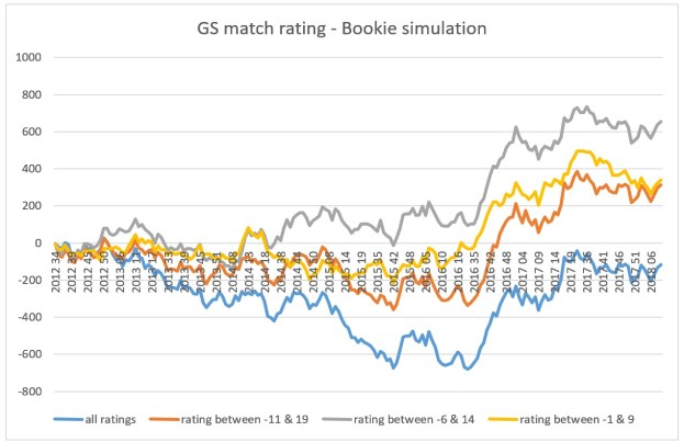
So would I recommend this model for professional sports betting? Definitely not! If you take a look at profit per season, you realise, that nearly the whole profit is generated in season 2016/17. Overall the model got a yield of 5,5%. Without season 2016/17 the yield decreases to 0,4%. The profits of each season more or less correspond with the observed accuracy. In 2016/17 the GS match rating model got nearly the same accuracy as the Bookie. But even if the accuracy for every other season was worse, the model did not produce the huge lose, which I expected. This again shows, that an accuracy based on the geometric mean does now allow conclusions to the profitability against the bookie.
The SQL source for the Bookie simulation can be found at GitHub:
GitHub – GS match rating Bookie simulation
Conclusion
Based on the GS match rating provided by football-data.co.uk and the self introduced PPG match rating this series showed how to optimise and compare different models, as well as test their profitability. Both models did not show the possibility to beat the bookie. So the next step of development process, the implementation of the model, can be skipped. This is perfectly normal as not each new model can be an improvement. And I already did not expect these models to be better than my Poisson model. But of course there are some things I learned during the optimisation.
(1) One-vs-rest for binary classifiers
The one-vs-rest strategy works really good for multi-class predictions with binary classifiers. As you need multiple models for each class and need to adapt the overall probabilities, the handling might not be the easiest one. But it offers the possibility using every binary classification method to predict the outcome of a football match or other multi-class prediction problems.
(2) Be aware of R-squared significance!
R-squared is meant to be as an indicator, how well a regression does fit the observed predictor variables. But as the comparison between the regression models showed, a higher R-squared does not always indicate the better predictive model. The PPG match rating polynomial regression model offered the best R-squared value, but also one of the worst accuracies.
(3) Accuracy != profitability
The geometric mean as an accuracy method does only use the predicted probability of the observed outcomes to calculate the overall accuracy of predictive model. This is not enough to get an estimation, whether a model will gain profit again the Bookie. The accuracy of the GS match rating model gives the impression, that the model would provide a loss every season. But instead the simulation results were not so bad. The leads to one conclusion: I have to look for another accuracy method, which more indicates the profitability of a predictive model.
If you have further questions, feel free to leave a comment or contact me @Mo_Nbg.
