
The first part of this series covered the definition of the network architecture for my Team Strength MLP. This neural network must now be trained. To explain and visualize the training process, Tensorflow offers the web frontend TensorBoard. This post will explain, how you use TensorBoard and what are some basic indicators for a well-trained model.
Executing TensorBoard
TensorBoard is automatically provided with Tensorflow. So there is no need to install any additional package. To start TensorBoard you just need to execute following command inside your Anaconda environment:
(tensorflow) C:>tensorboard --logdir c:/temp/tensorflow/output/logs/
The logdir parameter specifies, where TensorBoard expects the output of the Tensorflow training process. To enter the web front end of TensorBoard, you just need to call the URL throw your browser, which is shown, after you started TensorBoard.

Train a Tensorflow MLP
In order to provide the training output to TensorBoard and monitor the training process, you have to specify the output directory during the model definition.
#define model
model = tflearn.DNN(v_net,
tensorboard_dir='c:/temp/tensorflow/output/logs/',
tensorboard_verbose=0)
The parameter tensorboard_dir has to be the same directory mentioned at the start of Tensorboard. The tensorboard_verbose level defines, how much information should be logged during the training process:
- 0 – loss, accuracy (best speed)
- 1 – loss, accuracy, gradients
- 2 – loss, accuracy, gradients, weights
- 3 – loss, accuracy, gradients, weights, activations, sparsity (best visualization)
I started with verbose level 0 as I first have to learn, how to interpret the output for the other values. But this is definitely enough to get a basic feeling, whether your training process looks good or not.
To start the training process for your network, you have to call the fit() function of your defined model, provide the training and validation set, and pass some more parameters:
#train model
model.fit(df_x_train.values, df_y_train.values,
n_epoch=500,
batch_size=10,
show_metric=True,
validation_set=(df_x_val.values,df_y_val.values),
shuffle=None,
snapshot_step=100,
snapshot_epoch=False,
run_id = 'relu_adam_001')
The number of epoch determines how often the complete training data set is send through the network. One epoch is done throw several batches, whose size is specified throw the batch size. Both parameters effect, how often the weights of the neural network are adapted via back-propagation and therefore. how often the network learns the relationship between the input and output.
Monitor training process
As soon as you start executing the python code and start the training process, Tensorflow logs every output to the output directory and you are able to monitor the training process with TensorBoard. I cannot stress enough to just play around with all the parameters of your model a little bit at the beginning and look, which influence the different changes have to the training process. By doing this, I could collect some basic insights for training such a basic MLP.
Does my network learn something?
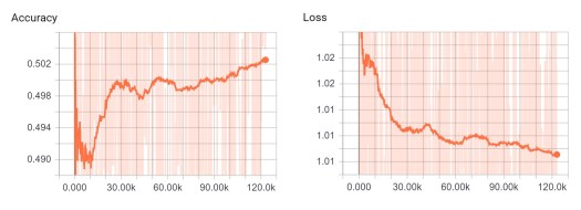
This question seems simple, but for me this was really a problem, when I tested some deep learning packages for R. I trained a model and recognized throw the prediction, that it learned nothing. But I did not know why and I was also not able to find out why. This was really frustrating. The graphical illustrations of Tensorboard helps a lot! You simply have to look for an increasing accuracy and a decreasing loss.
During testing different optimizers, activation functions and architectures with multiple hidden layers I recognized, that it can take while, until the learning process starts. So you maybe have to experiment with various number of epochs and batch sizes.
Choose the correct learning rate!
The learning rate has a huge impact on how fast your network learns. A very small learning rate causes a really slow learning process. In comparison a very high learning rate could provoke your model not to find the best accuracy and really “jump” over that point.

I always tried to adapt to the green and red line of the above illustration. This was a good compromise between learning speed and the risk to miss the best accuracy.
Identify Overfitting!
Overfitting is the typical problem, when the neural network memorizes the training data set. For a good generalization the accuracy of the training set and the validation set should be almost equal. A clear indicator for a overfitted model is a further on increasing training accuracy and a decreasing validation accuracy as presented by the blue line. Simultaneously you should see an increasing validation loss.

Using different parameters and network architectures showed, that the test and validation accuracy can differ a lot, but show the same trend, similar to the red and green line. This was mainly caused by a combination of two facts:
- the accuracy for a football prediction is in general not very high
- I just used 10% of my data set for validation
It happened, that the accuracy for the validation set was 4%-5% lower or even higher than the training accuracy. But the accuracy and loss graph did not indicate an overfitting. This problem was really random based on the splitting of the validation set. Increasing the validation set to 20% reduced this effect. As long as there are no other indicators for a overfitted model, an accuracy difference between test and validation is acceptable.
Save trained model
After your model is trained and you are happy with the different graphs for accuracy and loss, you can save the model.
#save the model
model.save('C:/temp/Tensorflow/v01/trained_model/relu_adam_001.tf_model')
At this point the model is just saved after all epochs have finished. You are also able to define an early stopping, when e.g. a specific validation accuracy is reached. Or you just save every checkpoint with a minimum accuracy in a pre-defined directory, which is part of the model definition.
This saved model will be the starting point for the 3rd part of the series. I will explain, how you reload such a trained model and predict the results for upcoming matches. After that, this knowledge can be used to back test the model and determine the real prediction accuracy for future datasets.
If you have further questions, feel free to leave a comment or contact me @Mo_Nbg.
References:
[1] Sagar Sharma, Epoch vs Batch Size vs Iterations, 2017, https://towardsdatascience.com/epoch-vs-iterations-vs-batch-size-4dfb9c7ce9c9
[2] Hafidz Zulkifli, Understanding learning rates and how it improves performance in deep learning, 2018, https://towardsdatascience.com/understanding-learning-rates-and-how-it-improves-performance-in-deep-learning-d0d4059c1c10

One Reply to “”