Validate model: Poisson distribution (part 1)

The first model I tested is based on the predictive models of Maher [1] and Dixon / Coles [2]. Maher modelled the expected goals for a specific match as two independent Poisson distributions. After that, Dixon / Coles improved this model to balance some disadvantages.

In the previous post I described, how you can easily calculate the features of these models for any football match in the past. The first part of this post will show you, how to calculate the odds with the help of these features and why a simple Poisson distribution is not enough to beat the bookie. How I solved these problems will be the central element of the second part.

Poisson distribution

According to Wikipedia the Poisson distribution “is a discrete probability distribution that expresses the probability of a given number of events occurring in a fixed interval of time and/or space if these events occur with a known average rate and independently of the time since the last event.” When we talk about events in football, we of course talk about goals in this context. So we use the Poisson distribution to calculate the probability for a specific number of goals a team shoots or concedes.

The probability of events is described by the equation:

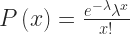
The equation for the Poisson distribution is really simple. There are only 2 parameters. X represents the number of goals (e.g. 0, 1, 2, …) a team shoots during a game.  represents the average number of goals expected during a game.

So let’s take a look at the Bundesliga: Between 2011 and 2016 an average of 2.89 goals were scored. Using this average with the Poisson distribution results in following probabilities:

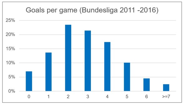
The probability that a game ends with zero goals is about 7%. Nearly 25% of games should end with 2 goals. But this is of course nothing we can use to forecast the result of a game as the distribution is calculated with the league average number of goals.

Expected goals

To predict the result of a single game, you have to calculate the expected goals for the home and the away team. All we need are the features described in Define variables: attack & defence strength:

The expected goals for the home and the away team can then be used to describe two independent Poisson distributions.

Here is a small example:

Bayern Munich played against Schalke 04 last season on February 4th. At this point the table for the attack and defence strength provides following performance figures.

Home team performance figures:

• League statistics:
  • Avg League Home Goals Scored: 1.58
  • Avg League Home Goals Conceded: 1.16
• Bayer Munich statistics:
  • Avg Home Goals Scored: 2.77
  • Avg Home Goals Conceded: 0.43
• Model features:
  • Home Attack Strength: 1.75
  • Home Defense Weakness: 0.37

 

Away team performance figures:

• League statistics:
  • Avg League Away Goals Scored: 1.19
  • Avg League Away Goals Conceded: 1.5
• Schalke 04 statistics:
  • Avg Away Goals Scored: 0.97
  • Avg Away Goals Conceded: 1.4
• Model features:
  • Away Attack Strength: 0.81
  • Away Defense Weakness: 0.93

Based on these figures you are now able to calculate the expected goals for the home and the away team.

Expected goals:

• Home Expected Goals: 2.57
• Away Expected Goals: 0.35

We can now use these expected goals for two separate Poisson distributions. This leads to following probability distribution.

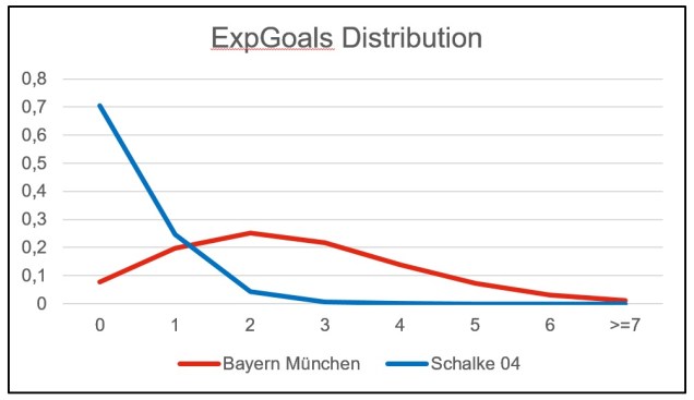
The final result of the game was a clear 3:0 home win for Bayern Munich. As you can see the probability for this result was the second highest. The final result 2:0 got the highest probability.

1×2 probabilities

As you can see in the example above, the usage of two independent Poisson distributions gives us the possibility to predict the probability of exact results. So if you want to calculate the probability of a home win, you just need to sum the probabilities of each possible home win result (e.g: 1:0, 2:0, 2:1, …). But how do you implement this calculation inside the existing DV Model?

At first,  you need a function, which implements the calculation of a Poisson distribution inside the database. Therefore, Exasol offers the so called User Defined Functions. Exasol supports native R code, which makes coding such a function very easy:

CREATE OR REPLACE R SCALAR SCRIPT analytical_layer.poisson ("p_x" DOUBLE, "p_mean" DOUBLE)
RETURNS DOUBLE
AS
run <- function(ctx)
{
   dpois(ctx$p_x, ctx$p_mean)
}

This function can then be used to create a new satellite table, which calculates, based on the attack and defence strength for a specific match, the expected goals for each team and the probabilities for a home win, draw and away win.

create or replace view analytical_layer.football_match_his_l_s_poisson_probs
as
select
  football_match_his_lid,
  round(home_attacking_strength * away_defence_strength * avg_league_home_goals_for,2) home_expect_goals,
  round(away_attacking_strength * home_defence_strength * avg_league_away_goals_for,2) away_expect_goals,
  round(analytical_layer.poisson(0, local.home_expect_goals),4) prob_home_0,
  round(analytical_layer.poisson(1, local.home_expect_goals),4) prob_home_1,
  round(analytical_layer.poisson(2, local.home_expect_goals),4) prob_home_2,
  round(analytical_layer.poisson(3, local.home_expect_goals),4) prob_home_3,
  round(analytical_layer.poisson(4, local.home_expect_goals),4) prob_home_4,
  round(analytical_layer.poisson(5, local.home_expect_goals),4) prob_home_5,
  round(analytical_layer.poisson(6, local.home_expect_goals),4) prob_home_6,
  1 - (local.prob_home_0 + local.prob_home_1 + local.prob_home_2 +
       local.prob_home_3 + local.prob_home_4 + local.prob_home_5 +
       local.prob_home_6)  prob_home_7,
  round(analytical_layer.poisson(0, local.away_expect_goals),4) prob_away_0,
  round(analytical_layer.poisson(1, local.away_expect_goals),4) prob_away_1,
  round(analytical_layer.poisson(2, local.away_expect_goals),4) prob_away_2,
  round(analytical_layer.poisson(3, local.away_expect_goals),4) prob_away_3,
  round(analytical_layer.poisson(4, local.away_expect_goals),4) prob_away_4,
  round(analytical_layer.poisson(5, local.away_expect_goals),4) prob_away_5,
  round(analytical_layer.poisson(6, local.away_expect_goals),4) prob_away_6,
  1 - (local.prob_away_0 + local.prob_away_1 + local.prob_away_2 +
       local.prob_away_3 + local.prob_away_4 + local.prob_away_5 +
       local.prob_away_6)  prob_away_7,
  round(
    local.prob_home_1 * local.prob_away_0 + --1:0
    local.prob_home_2 * local.prob_away_0 + --2:0
    local.prob_home_3 * local.prob_away_0 + --3:0
    local.prob_home_4 * local.prob_away_0 + --4:0
    local.prob_home_5 * local.prob_away_0 + --5:0
    local.prob_home_6 * local.prob_away_0 + --6:0
    local.prob_home_7 * local.prob_away_0 + --7:0
    local.prob_home_2 * local.prob_away_1 + --2:1
    local.prob_home_3 * local.prob_away_1 + --3:1
    local.prob_home_4 * local.prob_away_1 + --4:1
    local.prob_home_5 * local.prob_away_1 + --5:1
    local.prob_home_6 * local.prob_away_1 + --6:1
    local.prob_home_7 * local.prob_away_1 + --7:1
    local.prob_home_3 * local.prob_away_2 + --3:2
    local.prob_home_4 * local.prob_away_2 + --4:2
    local.prob_home_5 * local.prob_away_2 + --5:2
    local.prob_home_6 * local.prob_away_2 + --6:2
    local.prob_home_7 * local.prob_away_2 + --7:2
    local.prob_home_4 * local.prob_away_3 + --4:3
    local.prob_home_5 * local.prob_away_3 + --5:3
    local.prob_home_6 * local.prob_away_3 + --6:3
    local.prob_home_7 * local.prob_away_3 + --7:3
    local.prob_home_5 * local.prob_away_4 + --5:4
    local.prob_home_6 * local.prob_away_4 + --6:4
    local.prob_home_7 * local.prob_away_4 + --7:4
    local.prob_home_6 * local.prob_away_5 + --6:5
    local.prob_home_7 * local.prob_away_5 + --7:5
    local.prob_home_7 * local.prob_away_6 --7:6
  , 4) prob_home_win,
  round(
    local.prob_home_0 * local.prob_away_0 + --0:0
    local.prob_home_1 * local.prob_away_1 + --1:1
    local.prob_home_2 * local.prob_away_2 + --2:2
    local.prob_home_3 * local.prob_away_3 + --3:3
    local.prob_home_4 * local.prob_away_4 + --4:4
    local.prob_home_5 * local.prob_away_5 + --5:5
    local.prob_home_6 * local.prob_away_6 + --6:6
    local.prob_home_7 * local.prob_away_7 --7:7
  , 4) prob_draw,
  round(
    local.prob_home_0 * local.prob_away_1 + --0:1
    local.prob_home_0 * local.prob_away_2 + --0:2
    local.prob_home_0 * local.prob_away_3 + --0:3
    local.prob_home_0 * local.prob_away_4 + --0:4
    local.prob_home_0 * local.prob_away_5 + --0:5
    local.prob_home_0 * local.prob_away_6 + --0:6
    local.prob_home_0 * local.prob_away_7 + --0:7
    local.prob_home_1 * local.prob_away_2 + --1:2
    local.prob_home_1 * local.prob_away_3 + --1:3
    local.prob_home_1 * local.prob_away_4 + --1:4
    local.prob_home_1 * local.prob_away_5 + --1:5
    local.prob_away_6 + --1:6
    local.prob_home_1 * local.prob_away_7 + --1:7
    local.prob_home_2 * local.prob_away_3 + --2:3
    local.prob_home_2 * local.prob_away_4 + --2:4
    local.prob_home_2 * local.prob_away_5 + --2:5
    local.prob_home_2 * local.prob_away_6 + --2:6
    local.prob_home_2 * local.prob_away_7 + --2:7
    local.prob_home_3 * local.prob_away_4 + --3:4
    local.prob_home_3 * local.prob_away_5 + --3:5
    local.prob_home_3 * local.prob_away_6 + --3:6
    local.prob_home_3 * local.prob_away_7 + --3:7
    local.prob_home_4 * local.prob_away_5 + --4:5
    local.prob_home_4 * local.prob_away_6 + --4:6
    local.prob_home_4 * local.prob_away_7 + --4:7
    local.prob_home_5 * local.prob_away_6 + --5:6
    local.prob_home_5 * local.prob_away_7 + --5:7
    local.prob_home_6 * local.prob_away_7 --6:7
  4) prob_away_win
from
  analytical_layer.football_match_his_l_s_attack_defence_strength

The satellite table calculates the probabilities for the different number of goals a team can score. The upper bound is 7 goals. The probability for 7 goals sums up the probability for 7 or more goals. The second part of the satellite calculates the probabilties for a home win, draw and away win.

If we now select the probabilities for our example, these are the most likely results:

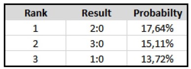
The odds for the 1×2 betting market look like this:

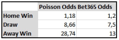
So the Poisson prediction model and Bet365 predicted a clear home win for Bayern Munich. The odds are also very similar, which is a good indicator for the prediction model. But would we bet such a bet? No! The predicted probability is greater than the implied probabilty of the betting odds and that’s why the bet has no value.

Model simulation

As you now got a satellite table with the predicted odds for every match in the past, you are now able to simulate these predicted odds against the historic odds of the bookie.

I decided to simulate following betting markets:

• Back Home / Lay Home
• Back Draw / Lay Draw
• Back Away / Lay Away

The odds for the back markets are available with the base data. The odds for the lay markets have to be calculated. These are just the inverse probabilities. But you have to take into account the margin of the bookie.

Following criteria were chosen to identify bets to play:

• Value > 0.2
• Probability > 0.1

The value of a bet has to be larger than 20%, because a small value could also just be a little inacccuracy. The event should have a minimum probability of 10%, so that the odds do not get too risky. I have selected these criteria only based on personal experience and testing.

Following graphs show the betting simulation for the 5 big European leagues:

 

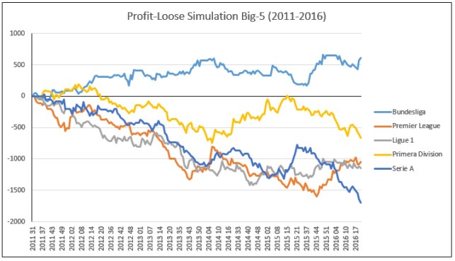
As you can see, the simulation looks not really good. The simulations for England, Spain, France and Italy end with a huge loose. Only the German Bundesliga provides a profit. But the graph of this simulation looks also not very satisfying. The graph does not show a steady profit. It is more an up and down. Some seasons provide profit, other seasons very little profit or loose.

Disadvantages of Poisson distribution

But why does the Poisson distribution not provide the possibility to beat the bookie? There are many sites in the internet, which suggest using a Poisson distribution to predict football scores. And the predicted probabilities for single matches look really good in comparison to the odds of the bookie.

The main problem is the Poisson distribution itself. The Poisson distribution expresses the probability for a given number of events, which happen independently. But goals in a football game usually do not happen independently. Goals have always e.g. a psychological effect on both teams. But this is something, which cannot be changed, when using such a model. There are leagues (e.g. Bundesliga), which better suite a Poisson distribution, and leagues (e.g. Serie A), which do not suite a Poisson distribution.

But there are also some disadvantages, which can be solved:

• Zero goals for a team are underestimated
• Draws are underestimated

 

In the second part of this post, I will describe, how you can solve these problems. This will not change the Poisson distribution to an ultimate model to beat the bookie, but it provides one stable prediction model.

 

 

If you have further questions, feel free to leave a comment or contact me @Mo_Nbg.

References:

[1]  Mike J. Maher. Modelling association football scores. Statistica Neerlandica, 36(3):109–118, 1982

[2] Mark J. Dixon and Stuart G. Coles. Modeling association football scores and inefficiencies in the football betting market. Applied Statistics, 46:265–280, 1997.