Validate model: Poisson distribution (part 2)

In the first part of this post I described, how a Poisson distribution can be used to predict football scores and why it is not sufficient to beat the bookie. The second part will now explain, how I balanced the disadvantages of the poisson distribution. This turned the model to an efficient predictive model, which can be used to gain profit against the bookie.

Disadvantages of the Poisson distribution

As mentioned in the last post, the main problem, while predicting football scores with the Poisson distribution, is the distribution itself. The distribution is a discrete distribution for independent events. But goals in a football match are not independent. Therefor using a better distribution would be the best choice, but this is not the goal for this prediction model. I  want to rebuild the model of Dixon & Coles.

So I tried to balance the other disadvantages of the Poisson distribution. A Poisson distribution underestimates the probability of low scoring games, especially zero goals and low scoring draws.

 

Zero Inflated Poisson distribution

To balance the underestimation of zero goals, I switched the used distribution to a Zero-inflated Poisson distribution. The Zero-inflated Poisson model consists of two components. One component for the probability calculation for zero events and the second component for all other number of events:

is the only new parameter of the distribution.  represents the probability for extra zeros. Following picture shows the difference between normal Poisson distribution and the ZIP distribution for the goal distribution in the Bundesliga during 2011 and 2016:

As you can see, the ZIP distribution provides a higher probability for zero goals, which is the goal for this optimisation. The probability distribution for 1,2 and 3 goals looks not perfect. But as mentioned, the Poisson distribution is per definition not the perfect distribution to predict the number of goals during a football match.

The calculation of the ZIP distribution can be, as for the normal Poisson distribution, implemented as a User Defined Function inside the Exasol database. The R Package VGAM offers the function DZIPOIS, which can be used to calculate the probability distribution. The UDF would look like this:

GitHub – UDF R Zip calculation

Unfortunately I am currently not able to upload the VGAM package into the Exasol database. As soon as I was able to do this, I will write a separate post, how to extend the R functionality of the Exasol database.

So I had to implement the ZIP distribution manually. Therefor you need 2 UDFs. The first on calculates the factorial:

GitHub – UDF factorial calculation

The second UDF implements the 2 components of the ZIP distribution:

GitHub – UDF Zip calculation

As already mentioned, the ZIP distribution needs an additional parameter: the extra probability for zeros. I have chosen following way to calculate this parameter: First I identify the percentage of home/away games with zero goals for the specific league. After that I can determine the difference between the Poisson-predicted zero goal probability for the home / away team and the observed percentage of the league. The result is used as the parameter for the ZIP function. I do not know, whether – from a statistical point of view – this is the correct approach. But for me it worked. If anyone know, how the parameter can be calculated in a better way, please leave a comment.

To determine the extra probability of zeros, the feature satellite described in Define variables: attack & defence strength has to be extended. The new satellite definition looks like this:

GitHub – Historic attack defence strength satellite

At lines 75-78 and lines 147-149 the original statement was extended to calculate the number of zero goal matches for the home and the away teams. The new columns are now useable for the calculation of the Zero-inflated Poisson distribution.

Draw correction factor

Switching to the Zero-inflated Poisson distribution should balance the underestimation of zero-goals matches. The next step of the model optimisation is to balance the underprediction of draws. Therefor I used the historic eventbased statistics for every team differed by home and away performance. Calculating the eventbased statistic is really simple. It is just the percentage of home-wins, draws and away wins for a specific number of past matches. The eventbased probabilities are defined as another satellite for the historic match link with following structure:

GitHub – Historic eventbased probabilities satellite

The statement consists of 3 parts. One part calculates the event probabilities for the head2head match history. The other two parts calculate the probabilities for the home team and the away team. For the head2head statistics a maximum number of 10 historic matches is used. A maximum number of 25 matches is used for the home and away statistics. In the result set the home and away probabilities get combined to the historic probabilities. This is the feature, which I used as the correction factor to balance the predicted draw probability.

1×2 ZIP probabilities

In the same way I created a new Satellite table with the 1×2 probabilities for the Poisson distribution in the first part of this post, I created a Satellite for the Zero-inflated Poisson probabilities. There is just one little difference: As mentioned before, I use the eventbased probabilities as a correction factor. So, there are now 2 possibilities. First you could already pay attention to the correction factor inside the ZIP probabilities Satellite. But by doing this, you have to be sure, which ratio you want to use. The second option is, to include the correction factor only when simulating the model. This is the option I have chosen, because so I am able to change the ratio easily, while testing the model. The Satellite table for this option looks like this:

GitHub – Historic ZIP probabilities

If you compare the structure to the Satellite table for the Poisson probabilities, they look really similar. The only difference between these two is, that the additional parameter for the Zero-inflated Poisson distribution has to be calculated and used during the UDF call. Otherwise the logic is the same. The probability for a specific event (home win, draw, away win) is calculated by summing the probabilities for the different results, which belong to this event.

Model simulation

With the new satellite tables the optimisation of the predictive model is finished and the optimised model can be simulated to check, whether the improvements achieve the desired effect. The predictive model now has following variable parameters, which can be adjusted to influence the result of the model:

Number of historic matches for attack / defence strength

The historic attack defence strength satellite uses a defined number of historic matches to calculate the attack and defence strength for the home and away team. This parameter can be changed while creating the satellite. If you choose a smaller number of matches, the attack & defence strength adapt faster to a improved or declined team performance. If the number of historic matches is larger, the strength features adapt slower. I have chosen the value based on some personal tests.

Chosen Value: 30 matches

Number of historic games for eventbased probs

The same applies to the determination of the eventbased probs. This satellite uses also a specific number of historic matches to calculate the eventbased probs for the home / away team and another number of historic matches to calculate the probabilities for head2head matches. The number for the head2head matches has to be small, as there can only be 2 direct matches between 2 teams during a season. I adapted these values from another blog, where these features were used, to roughly calculate the probabilities for different match results.

Chosen Value: 25 matches for home / away probs, 10 matches for direct probs

Ratio of correction factor for draw games

The eventbased probabilities get used as a correction factor during the calculation of the fair probabilities for a match result. So you have to specify, how big the influence of the correction factor should be. During the simulation of the model I just tested different values for this parameter, to see which value works best.

Chosen Value: 0,3 

Filter for value

The value of a single bet shows the difference between the probability expressed by the betting odds and the predicted probability. Of course you need a positive value to make profit. A small value indicates, that there is nearly no difference between the predicted probability and the betting odds. A huge value could represent two facts: Either the bet is really underestimated or the prediction model is inaccurate. This value was also just determined during the simulation.

Chosen Value: > 0,2

Filter for bet probability

I decided to add also a filter for bets with a specific bet probability. I recognized, that some betting odds occur very rarely. Because of this, the law of small numbers could cause, that you make a big loose before even one bet wins.

Chosen Value: > 0,1

With these parameters you can now simulate the improved model. Following graphs show the betting simulation for the 5 big European leagues:

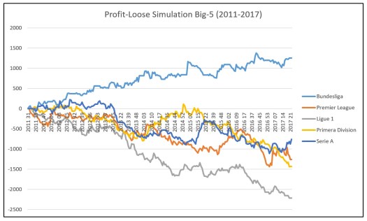
Serie A simulation improved a lot, but still provides a loose. But for the German Bundesliga the desired improvement can be seen. The profit loose graph looks much more steady. A look at the yearly profit confirms this:

So the model provides a yearly profit. Overall the model provides a yield of 6.8% over a total number of 1853 bets. From my point of view, this looks really good.

But this not only a simulation of the past. I developed the model during the season 2016/17 and started to populate picks in February 2017. So the simulation of the last season is also a prove for the populated picks.

In the last post for this predictive model, I will explain, how you implemented the prediction for the current matches and what structure the report has, where the whole information of the model gets combined. I will also populate a post, where I describe, how I simulate predictive models.

 

 

If you have further questions, feel free to leave a comment or contact me @Mo_Nbg.

 

References:

[1]  Mike J. Maher. Modelling association football scores. Statistica Neerlandica, 36(3):109–118, 1982

[2] Mark J. Dixon and Stuart G. Coles. Modeling association football scores and inefficiencies in the football betting market. Applied Statistics, 46:265–280, 1997.