Inflated ML Poisson model to predict football matches

My last blog post “Poisson vs Reality” did change something in my head. I realized, that I not yet checked single parts of my model enough, whether they differ from reality and whether I could reduce this difference and improve the model performance. That’s why I started creating a new model approach for the new season and focus on the improvement of single steps during the model process. After the training of multiple models, I will test against the fair profit, which kind of adaptions improve a Poisson distribution model the most.

First let’s have a look at my new model approach. I really like the method using a Poisson distribution to predict football matches. [1] Getting the single probabilties for the number of goals a team could score, makes it really easy, to create the probabilities for multiple markets. On the other side, a classic Dixon&Coles model is limited, as you are just able to use goals or xGoals as features for the model. But I really like to add and test multiple features for a model, as there are many statistics, which have a big influence on the result of a football match. So I decided to make it a bit different this time. I am using a machine learning regression model to predict the ExpectedGoals for the home and away team of a match and test different sets of features. After this I use these predicted ExpectedGoals for two independent Poisson distributions. So I am able to use the advantages of both approaches.

Model process

To spot possible options where to improve or adapt the model, I took a look along the whole model process. At some points, there is just the possibility to use different options and look, which one provides the better performance. For other steps I am able to compare an intermediate result with the reality. If I spot a difference, I might be able to improve the model there. With respect to the reading time of the article, I will not make a deep dipe into the technical implementation of the single steps.

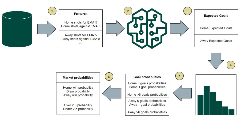
1 Feature calculation

At first I need to select the features, which are used for the machine learning model to predict the expected goals. These features get aggregated as an exponential moving average (EMA) so that the latest matches have a higher weight. For the number of past matches, which should be used for the EMA calculation, I defined 4 different time windows: the last 5, 10, 15 or 20 matches. Each type represents a single model.

Statistic	Features calculated for home & away team for the last X matches
Goals	Goals for, Goals against
xG	xG for, xG against
Shots	shots for, shots against
Shots on target (SoT)	SoT for, SoT against
Corner	Corners for, Corners against
Deep	Deep passes for, deep passes against
Passes per defensive action (PPDA)	PPDA for, PPDA against

The home advantage in football is well known. That’s why it’s a common method to use just the home matches to calculate the home features. When using both, home and away, you should think about adding a home advantage factor. As I am using a machine learning model, I don’t have to care so much about this. Nevertheless I want to test both featue types.

Feature type	Feature calculation
COMB	Performance of the last home and away matches are used for the feature calculation
HA	Only the last home matches are used for the feature calculation of the home team and vice versa for the away team

Feature selection is an important method to improve the performance of a machine learning model. You reduce your overall amount of different features and specify specific features set to e.g. reduce the computing time or eliminate features, which just add noise to you model. I decided to not use a method to determine the feature sets. Instead I used logical selections. A full set and a set divided into relevant attack and defence features as well as a pure xG feature set, which are used by my Vanilla xG Poisson model.

Feature set	Included Features
FULL	The complete list of features is used. The home expected goals model and the away expected goals use all features for the home and away team.
HA	Contains also the complete list of features. The home expected goals models uses just the attack features of the home team and the defensive features of the away team. (e.g home goals for & away goals against). It’s the opposite for the away expected goals model.
XG	Only xG stats are used, similar to the classic Dixon&Coles approach. Again the home expected goals model does only use attack feature of the home team and the defensive feature of the away team.

So the first step in the model process already provides multiple different models. This number will now step by step increase, as I add more combinations.

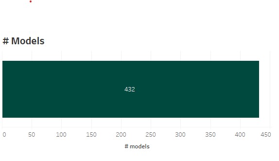
4 [different window sizes] * 2 [feature types] * 3 [feature sets] = 24 models

2 Machine learning model

The problem of predicting the ExpectedGoals for a match is a regression problem. Based on a set of variables, you want to predict another variable. Here I decided to test 2 different algorithms, which can be used for the such a regression problem: Random Forest Regressor, XGBoost Regressor [3]. I used both algorithms to train the different models. So we are already at an overall number of 48 models.

3 Expected Goals

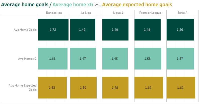
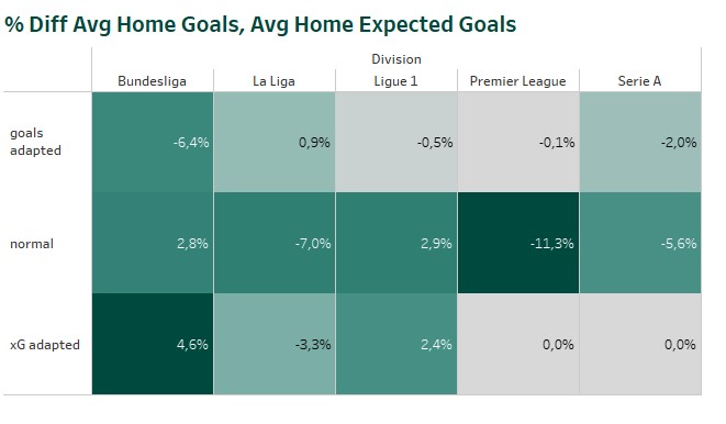
The home and away ML models provide the expected home and away goals for a single match. If the models would have a perfect accuracy, the average expected goals would be identical to the average scored goals. But that’s not the case. Comparing the average scored goals and xG, we can see some over- and underestimation. In case of Serie A the models overestimate the number of goals scored by the home teams (1.56) . It’s the same, when comparing the average expected number of home goals with the corresponding xG values. (1.57)

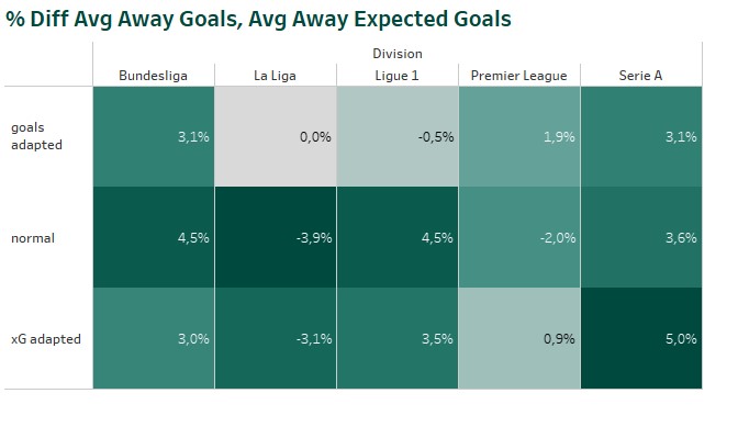
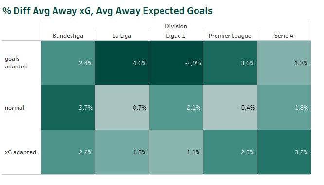
So I decided to test two optimization methods to reduce this difference. That’s done by determine the difference between e.g. the scored and expected home goals of the last 100 matchdays of the division before the match. The expected number of goals for the single match gets inflated or deflated based on this percentage value. The adaption is done in two different ways. First, based on the number of scored goals (“goals adapted“). Second, based on the number of xG (“xG adapted“).

[Adapted exp home goals] = [Exp home hoals] * ([Avg home goals / xG last 100 matchdays per division] / [Avg expected home goals last 100 matchdays per division])

[Adapted exp away goals] = [Exp away goals] * ([Avg away goals /xG last 100 matchdays per division] / [Avg expected away goals last 100 matchdays per division])

As expected the methods reduced the difference between the ExpectedGoals and the league averages. Inflating or deflating the single predictions based on xG reduces for most of the divisions the difference to the average xG scored in the past. The optimization based on scored goals, reduces the difference between average scored goals and average expected goals. Whether one of the optimizations improves also the overall profit of a model, will be shown during the model simulations.

4 Poisson distributions

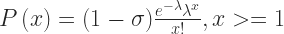
As described in the classical Dixon&Coles approach [4] the predicted ExpectedGoals are used for 2 independent Poisson distributions – one for the home team and one for the away team. The Poisson distribution returns the probability of a team scoring 0,1,2, … goals in a match.

5 Goal probabilities

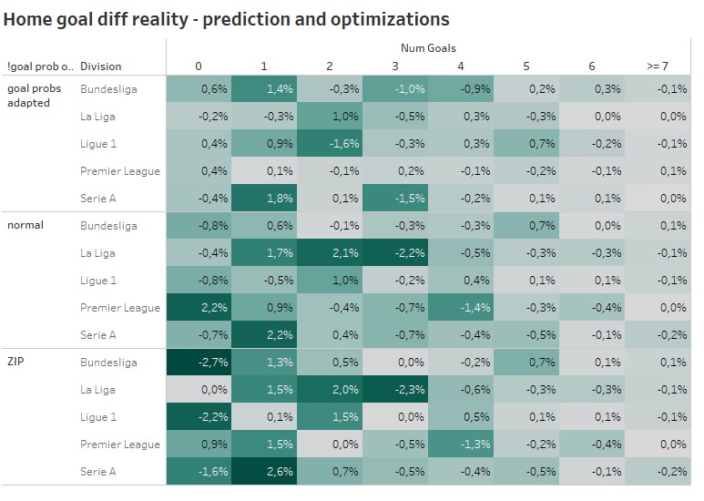
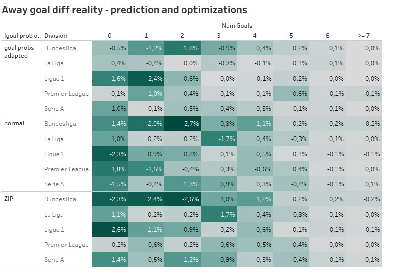
In one of my last blog post, I already explained some disadvantages of the Poisson distribution. The resulting goal probabilities especially for the low number of goals, does not always represent the reality. Looking at the away goals distributions for Ligue 1 we can spot an overestimation of matches with 0 away goals. In the Bundesliga the away team scoring 2 goals is overestimated on average.

Again I decided to introduce 2 different improvements and try to mend these drawbacks. The first optimization is a well know old friend, the Zero-inflated Poisson (ZIP). I already used it for one of my first models. In comparison to the normal Poisson distribution an inflating parameter is used to adapt the probability for 0 goals. I used the difference between the expected percentage of matches with 0 goals and the real percentage of matches with 0 goals during the last 100 matchdays as .

With a 2nd different approach I tried to respect the fact, that also the probability for scoring e.g. 2 goals might need to be adapted (goal prob adpated). Therefor I determined the difference between the average predicted probabilities for e.g. matches with 0 home goals and the real distribution based on the last 100 matchdays of a division. So every single goal probability gets inflated or deflated.

[Adapted 0 home goal prob] = [0 home goal prob] * ([Avg pred probability for 0 home goals last 100 matchdays per division] / [# perc matches with 0 goals last 100 matchdays per division])

Even though the ZIP is the more traditional approach, which was used already in multiple papers about football predictions, the goal prob adaption approach seems to do a better job, when it’s about decreasing the difference between the average predicted and real goal distribution. For high scoring matches major adaptions were not needed and were also not done. For lower scoring games the lighter color for the goal prob adapted approach indicate a better reduction of differences.

6 Market probabilities

In the last step of the model process, the single goal probabilities get aggregated to the desired markets. In my case these are the 1×2 markets. The probability of a draw is the sum of all results with the same number of goals.

[draw prob] = ([0 home goals prob] * [0 home away prob]) + ([1 home goals prob] * [1 home away prob]) + ([2 home goals prob] * [2 home away prob])
 + ([3 home goals prob] * [3 home away prob])
 + ([4 home goals prob] * [4 home away prob])

Model simulation & profit

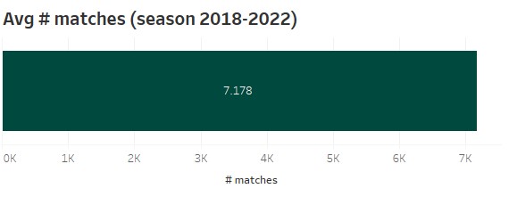
All the different model combinations result in an overall number of 432 different models. For the simulation of the models I used the Big5 leagues (Premier League, Bundesliga, Ligue1, Serie A) and the seasons 2018 – 2022. So every model betting simulation uses 7.178 matches on average.

In comparison to model simulations in older blog posts, I will from now on use the fair bet365 odds and calculate the past profit based on these odds. There are 2 reasons for this. On one side I still not trust the Brier score as an performance measure for betting models. On the other hand, using specific bookmaker odds, which include their margin, does not really help to get an impression about the potential of a model, as each bookmaker uses a different margin. How to calculate the fair odds, is described in my previous blog post.
Additionally there’s another adaption for my betting simulations. While analysing the problem of my different models, I recognized, that there’s really a problem, when it’s about Draw bets. That’s really a weak spot. So I decided to ignore Draw bets and tackle this problem separately.
Now let’s have a look, how the different model types and optimizations improve or influence the profit. Therefor I calculated the average profit for the single model characteristics. As I got such a big amount of models, this should provide a good indication, what kind of model should perform on average the best for future bets.

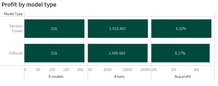
1 Machine learning model

As I only used 2 different ML algorithms, there are 216 different models for each. About 1.5 million bets were selected for each model type. On average the Random Forest provides a slightly higher average profit with 5,32% in comparison to 5,17% provided by the XGBoost models. So it’s already clear, that my final model will be based on a Random Forest.

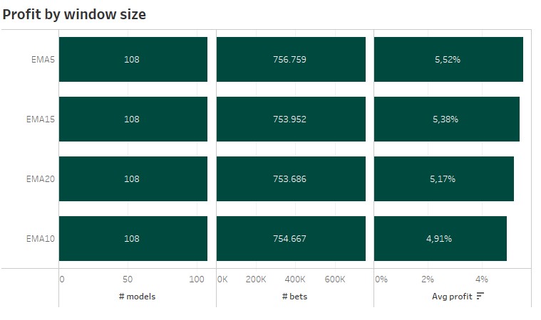
2 Window size

For each window size 108 models with around 750k bets are used. Surprisingly the shortest time window with 5 matches for the exponential moving average produced the highest average profit. Based on my past experience and the accuracy during the ML model training, I expected the bigger window sizes to perform best.

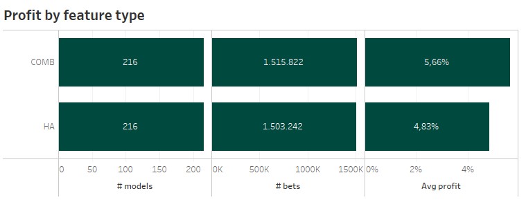
3 Feature type

There was no surprise looking at the two different feature types. One of my older blogs already indicated, that you do not need to differ between home and away performance, when using machine learning algorithms. Models using the combined features have a higher average profit.

4 Feature set

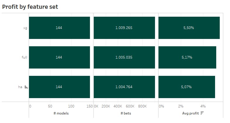
The feature sets revealed the next surprise. The simple xG features set, which is also used for my Vanilla Poisson xG models, performed best. I would have expected a feature set containing more features and also more information to be superior. This might also be a topic, which I should take a deeper look in a separate blog. The difference might look big, but when respecting the previous criterias, the difference get’s nearly non-existent.

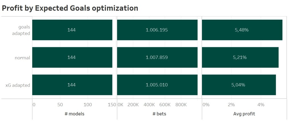
5 Expected goals optimization

Using the average number of home and away goals as an anchor to improve the predicted Expected goals values of the ML model improved the average profit the most. This optimization should be favoured, as the same approach using xG data even degrade the model performance.

5 Expected goals optimization

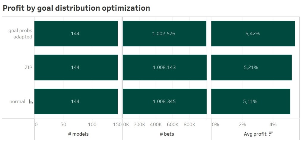
Again another surprise. The ZIP approach did not perform the best. Yes, it improves the models performance. But the average results based on 144 different model combinations indicate, that also for standard Poisson distribution you should inflate or deflate each goal probability with the average historic values.

Conclusions

So we got our winner. My model used for the new season will be a Random Forest model with just xG features based on a 5 matches expential moving average not splitted by home and away games, which gets improved by 2 goal-based optimization for the Expected goals and the overall goal distribution. But there are some more conclusions….

1. I am still surprised, how different the model performance looks like, when using the fair odds for a model simulation. I think, I will stick to this method for future back testing and model comparisons. Using the Brier score as an alternative is still not a option for me.
2. The new model approach shows a better performance than the Vanilla xG Poisson model and still provides some small aspects, which could be investigated a bit more. So more room for improvement.
3. Using average historic goal distributions as a kind of anchor reduced some inaccuracies in the predictions. Surprisingly the well-known Zero-inflated Poisson distribution seems not the best choice.
4. The advantage of multiple feature sets when using a ML model to predict the expected goals is really great. This should now also help to create a model for smaller leagues, where no xG data is available. Goals alone are unfortunately to noisy to create a good model.

If you have further questions, feel free to leave a comment or contact me @Mo_Nbg.

References:

[1] https://www.pinnacle.com/en/betting-articles/Soccer/how-to-calculate-poisson-distribution/MD62MLXUMKMXZ6A8

[2] https://www.pinnacle.com/en/betting-articles/Soccer/inflating-or-deflating-the-chance-of-a-draw-in-soccer/CGE2JP2SDKV3A9R5

[3] https://machinelearningmastery.com/xgboost-for-regression/

[4] Mark J. Dixon and Stuart G. Coles. Modeling association football scores and inefficiencies in the football betting market. Applied Statistics, 46:265–280, 1997.

https://mljar.com/blog/feature-importance-in-random-forest/#:~:text=Random%20Forest%20Built%2Din%20Feature%20Importance&text=It%20is%20a%20set%20of,sets%20with%20similars%20responses%20within.