
“Goals are the only statistic, which decide a match” – sentences like this appeared not only once, while reading discussion about the latest xG statistics of single matches on Twitter. Even if the statistic xG is more and more used by sport journalists and during broadcasts, the meaning and importance of the statistic is not yet widely understood. This might be caused by the usage of xG for single matches or single shots. The final result of a match and the corresponding xG values might differ a lot. But over the long-term xG is a statistic, which tells us way more about a football team than goals and shots alone. To prove this, this post will take a look at the predictive power of xG in comparison to goals. The more information a statistic contains the more it should help us to predict the result of future matches.
What are Expected Goals (xG)?
In my older xG data journey post, I already took a look at the definition and usage of xG. So instead of writing again many sentences about this statistic, you can just follow the link or maybe just watch again this video, which I think explains the base idea really good.
Which data is used?
To test the predictive power of xG statistics, we need a lot of data. In this case I used Understat data of the last 5 years for the Big5 in Europe. So we got something about 12.000 matches with goal and xG statistics.
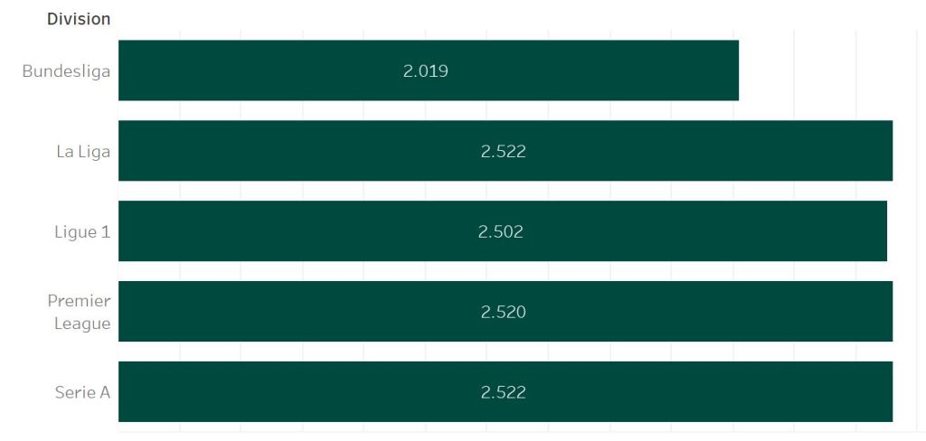
The different number of matches, while divisions containing the same amount of teams, is caused by the availability of predictive features. Promoted teams need a specific amount of matches before the features can be calculated.
As a benchmark for the predictive power the betting market will be used. Football-data.co.uk provides historic odds for a huge amounts of leagues. In an older post I already described how I used this data to build the base for my predictive system.
The Poisson model
The goal of this post is not to find a predictive model, that is able to beat the market. I just want to compare the usage of goals and xG stats in a predictive model. That’s why I decided to use a model, which I already used and is known to be able to calculate usefull predictions: the Poisson model. The model assumes that the result of a football match can be described by two independent Poisson distributions, which are based on the number of goals the home and away team are expected to score.
Model features
The number of expected goals for each team is calculated by the attack and defence strength. Because of the home advantage you have to differ between home performance and away performance
HomeExpGoals = HomeAttackStrength * AwayDefenceStrength * AvgLeagueHomeGoals

AwayExpGoals = AwayAttackStrength * HomeDefenceStrength * AvgLeagueAwayGoals
The different strength features are calculated by deviding the number of goals scored or conceded by the corresponding league average. So the features indicate the team strength in comparison to the league average. How much goals was a team able to score in comparison to the league average or how many goals did a team concede in comparison to the league average.
HomeAttackStrength = AvgHomeGoalsScored / AvgLeagueHomeGoalsScored

HomeDefenceStrength = AvgHomeGoalsConceded / AvgLeagueHomeGoalsConceded


AwayAttackStrength = AvgAwayGoalsScored / AvgLeagueAwayGoalsScored

AwayDefenceStrength = AvgAwayGoalsConceded / AvgLeagueAwayGoalsConceded
Simple Moving Average vs. Exponential moving average
My old Poisson model based on goals shows one big disadvantage: It reacts to slow, when a teams performance is strongly increasing or decreasing. That’s caused by the use of the Simple Moving Average (SMA), which does not weight the latest matches more than older matches. In comparison the Exponential Moving Average (EMA) uses an exponential weight ing for the latest matches. To also determine, whether this is also the case for a Poisson model based on xG data, I will test a SMA and a EMA Poisson model.
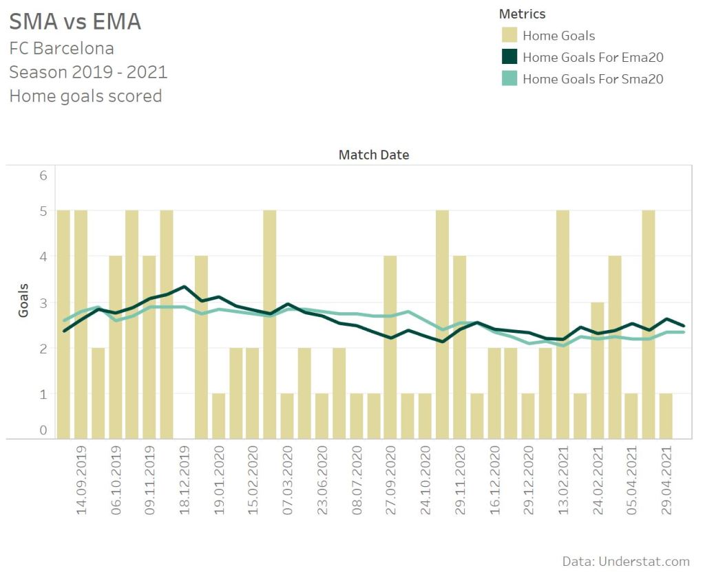
The dark green line represents the 20 matches exponential moving average. The light green line the simple moving average for last 20 matches. Between the start of 2020 and end of 2020 Barcelona scored less home goals. Until October you are able to see, that the EMA declines more than the SMA. The SMA stays nearly the same. In comparison the EMA starts above 3 goals per matches and declines under the SMA line. In comparison two home matches with 5 and 4 goals scored in November 2020 increased the EMA line directly. That’s the typical behaviour of a SMA and EMA. The simple moving average does not weight any match. So a good or bad phase 15 matches ago can still heavily influence the average. The exponential moving average directly reacts, if the latest results show a big change in comparison to older matches.
Time-window parameter
A second important parameter for calculating the strength features is the number of games you want to consider for the attack and defence strength. The less games you consider the faster and stronger a model reacts on a increasing or decreasing performance. The more games you consider, the more “calm” the model reacts. This fact is e.g. used for a MACD analysis, which I already used to analyse the performance of a football team.
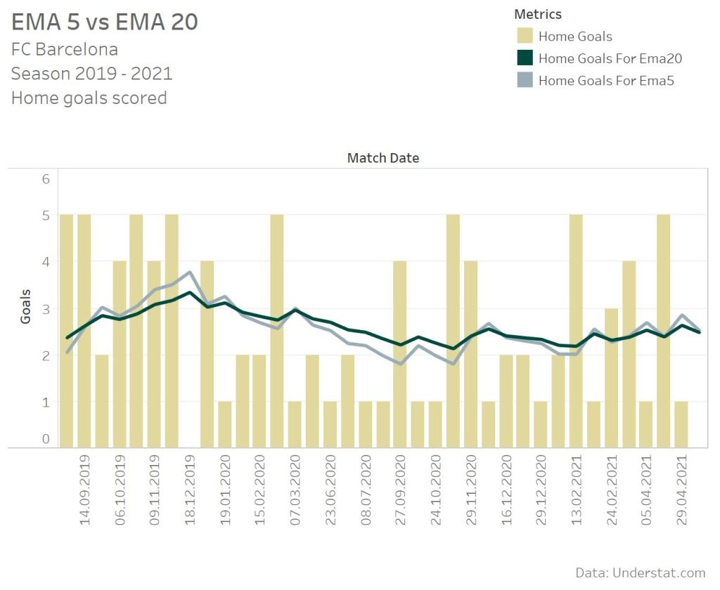
The graph again shows the same time period for the FC Barcelona. Looking at the 2 home matches in November 2020 clearly shows the difference between a 20 match history and a 5 match history. The EMA 20 already weights the latest game more and reacts more directly than the SMA. Changing the timespan to 5 matches even increases the effect, and the EMA reacts even harder on the increased performance in these two home matches.
The models
To test a wide range of short-term and long-term models, I decided to choose time windows from 5 to 35 matches. Combining this with the weighted and non-weigthed average results in 14 model combinations.
| # Matches | Non-weighted | Weighted |
| 5 | SMA 5 | EMA 5 |
| 10 | SMA 10 | EMA 10 |
| 15 | SMA 15 | EMA 15 |
| 20 | SMA 20 | EMA 20 |
| 25 | SMA 25 | EMA 25 |
| 30 | SMA 30 | EMA 30 |
| 35 | SMA 35 | EMA 35 |
Adding the fact that I want to test the different model combinations for goal and xG stats, these are 28 models overall. Such a wide range of different model parameter could also just be called a parameter optimization, because that’s basically the same, when you try to improve a model.
Feature calculation
Now it’s time to face the techical part of this blog and take a look at some of the technical implementations. I don’t want to go too much into details, because you can also find the complete source code at my GitHub repository.
In the 1st step the SMA and EMA for goals scored and conceded has to be calculated. Calculating the SMA is relative easy as nearly every database vendor offers analytical functions to calculate such sliding window averages.
avg(home_goals) over (partition by home_team order by match_date rows between 35 preceding and current row exclude current row) home_goals_for_sma35As a function the AVG is used to determine the average number of goals. The average is calculate over the HOME_TEAM partition to just get the number of goals the specific home team scored. The get a chronological sliding window everything is sorted by the match date. The size of the sliding window is defined by the ROWS BETWEEN clause. In this we take 35 preceding rows and exclude the current one. By doing this the average is calculated exactly up to the current match.
The EMA cannot be calculated with SQL functions. Therefor I used the Python Pandas function to calculate the EMA and created and Exasol UDF, which can be used in a SQL Statement. The EMA functions expects the team as a grouping parameter, the match date as the sort parameter and an integer value for the time span, which defines the sliding window.
select
  betting_dv.ema(home_team, match_date, home_goals_for, 35)
from
  home_his
group by
  home_team
For the attack and defence strength calculation the average number of goals scored and conceded is also needed. Here I don’t differ between SMA and EMA as a league average does not change so often over time. In this case the division itself is the partition criteria and a window size of 500 matches is used.
round(avg(home_goals) over (partition by division order by match_date rows between 500 preceding and current row exclude current row),1) home_goals_for_sma500As already described all these average features can now to be used to calculate the attack and defence strength features followed by the expected goals for the home and away team of a match. Based on the model parameters the expected goals for a single match can differ a lot. Let’s take a look at the match between Liverpool and Man City in the season 2020/21.
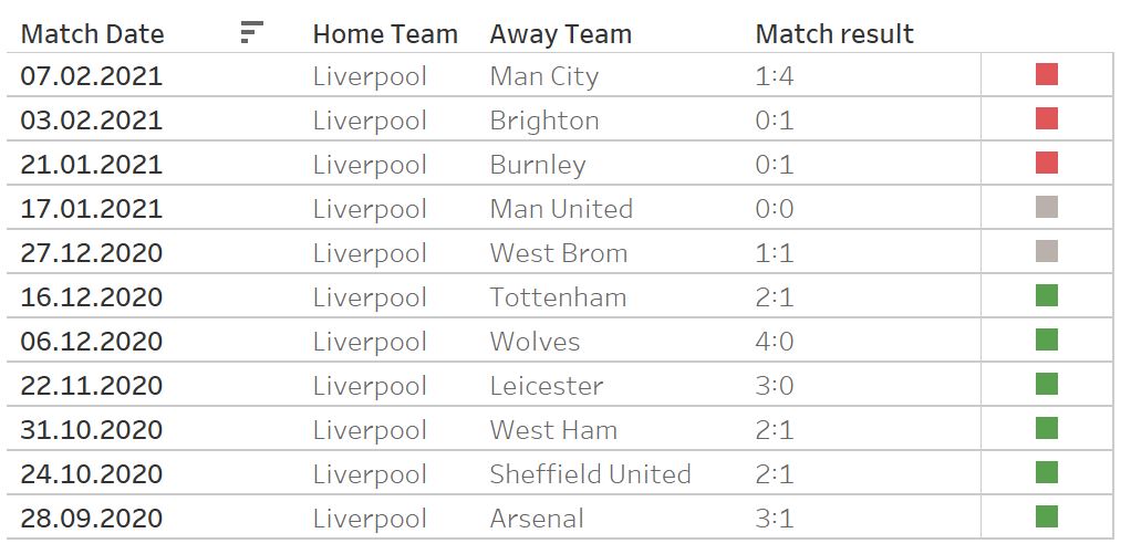
Since December 2020 Liverpool suffered a dramatic decrease in their home performance. After seeming almost unbeatable they drew two games and lost the next 2. This is also reflected by the expected goals values of the different models.
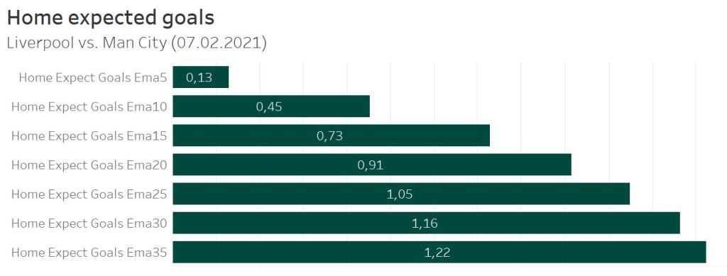
When only a time window of 5 matches is used to calculate the features, Liverpool was only expected to score 0.13 goals, as there was only one win in 5 matches before while scoring no goals the last 3 matches. The more matches are taken into account, the higher the number of expected goals gets, as more matches from the good-performing time window are part of the feature calculation.
Prediction results
As described by Maher [1] and Dixon / Coles [2] the used model assumes that the score probability in football follows a Possion distribution.

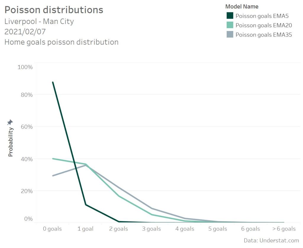
The Poisson UDF function returns the probability for a specific amount of goals based on the expected number of home goals or away goals. For the EMA and a 5 match history Liverpool was just expected to score 0.13 goals. This results in a probability of 88% to score zero goals and 11% to score 1 goal. In comparison with a 20 match history for the strength calculation Liverpool was expected to score 0.91 goals. This value shows a complete different Poisson distribution. In this case the probability of scoring no goals is descreasing to 40%.
The get the overall probability for e.g. a draw, the single probalities for the score lines (0:0, 1:1, 2:2, 3:3,… ) need to be summed up. Comparing all models for the Liverpool match shows a big difference in the home win probability. As expected the EMA5 model based on the actuals number of goals scored shows the lowest home win probability. The more matches are respected in the model, the higher the win probability as the good long-term performance of Liverpool is also considered. What’s the best number of historic matches to take care of in the calculation? That need to be tested with the overall accuracy of the different models, not on a single match base.
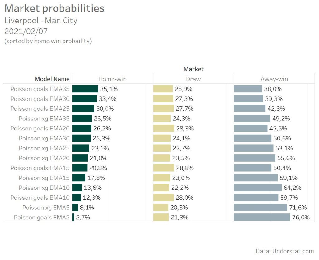
But the single match probs already reveal some interesting facts for the comparison of goals vs. xG models.
The goal models are at the extrem ends of the probability spectrum. They provide the lowest as well as the highest home-win probability. The difference between the Poisson goals EMA5 model and the Poisson goals EMA35 model is over 30%. The difference between the corresponding xG models is just over 18%.
Another finding are the different draw probabilities of the goals and xG models. The goal models suggest an average draw probability of 26,9%. The xG model have an average prob of 23%. Basic Poisson models are know for over- or underestimating the Draw probability [3], especially the 0:0. But that’s something, which has to be considered as a separate topic and will not be part of this post, as I just want to compare the base predictive power.
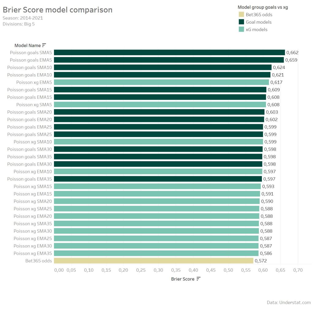
Model comparison
To compare and evaluate the different model, I will again use the Brier score, which I already used in some of my older Posts. The Brier score can be used for binary and multiclass classifications.

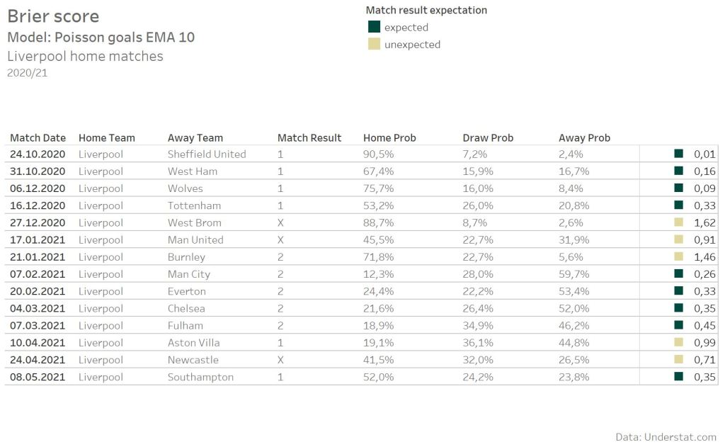
The lower the Brier score is, the more accurate was the prediction. In this case, a 3-class prediction (1×2), a Brier score lower than 0.66 can be assumed as a expected result. The higher the Brier score, the more unexpected a result was. The Poisson EMA 10 model creates relative extrem predictions caused by the small time window. That’s good as long as the prediction is correct. The home match against Sheffield United has a really low Brier score as the model was extremely “sure”, that Liverpool will win the match. But such extrem prediction can also cause the opposite effect, as e.g. the home match against Burnley shows.
The model with the lowest average Brier score provides the best accuracy for predictions. To also have some kind of benchmark value, I added the Bet365 odds. But as expected none of the models is able to beat the bookmaker model.
Overall it’s well recognizable, that the usage of xG over actual goals for such a simple Poisson model improves the predictive accuracy. The best xG model provides a Brier score of 58.6, while the best Goal model provides 59.7. Using the Bet365 odds Brier Score of 57.2 as the reference, that’s a over 40% improved Brier Score. Additionally the Top10 models are all xG models.
Something, what suprised me a bit is the influence of the EMA in comparison to the SMA. Models use time-dependent weighted parameter to improve the accuracy and weight the latest results more. But the effect seems less than expected. The difference between the corresponding EMA and SMA models is really small. The Top10 models consists of 5 EMA and 5 SMA models.
Once again, this post is not about finding a model, which is able to beat the Bookies and I also did not expect it. But having bookmaker odds as a reference is really helpful to get an estimation, how much better a predictive model with xG data gets.
Betting results
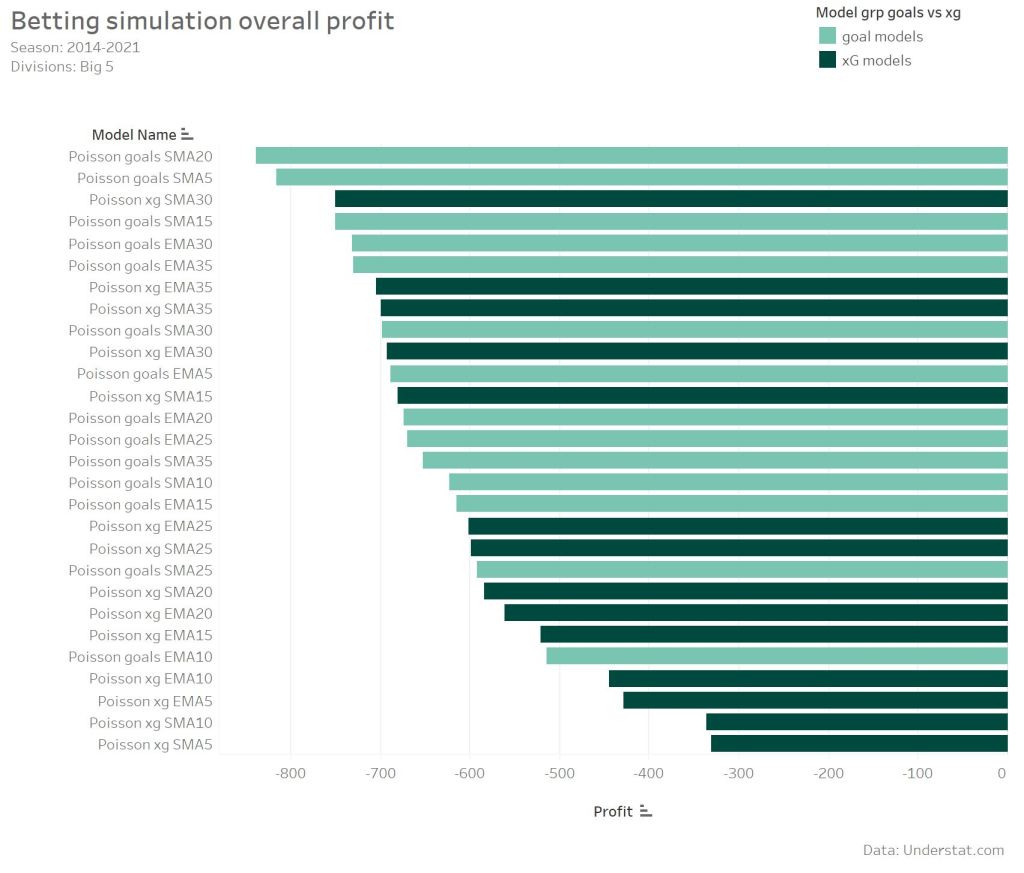
Beside knowing the Brier score for each model, it’s of course also interesting, how such a model performance against the betting market. Caused by the higher Brier score in comparison to the betting odds, it’s clear, that I am not expecting any profit. For the betting simulation only value bets a considered. A bet is considered a value bet, if the probability of a model for a specific match result is higher then the corresponding market odd.

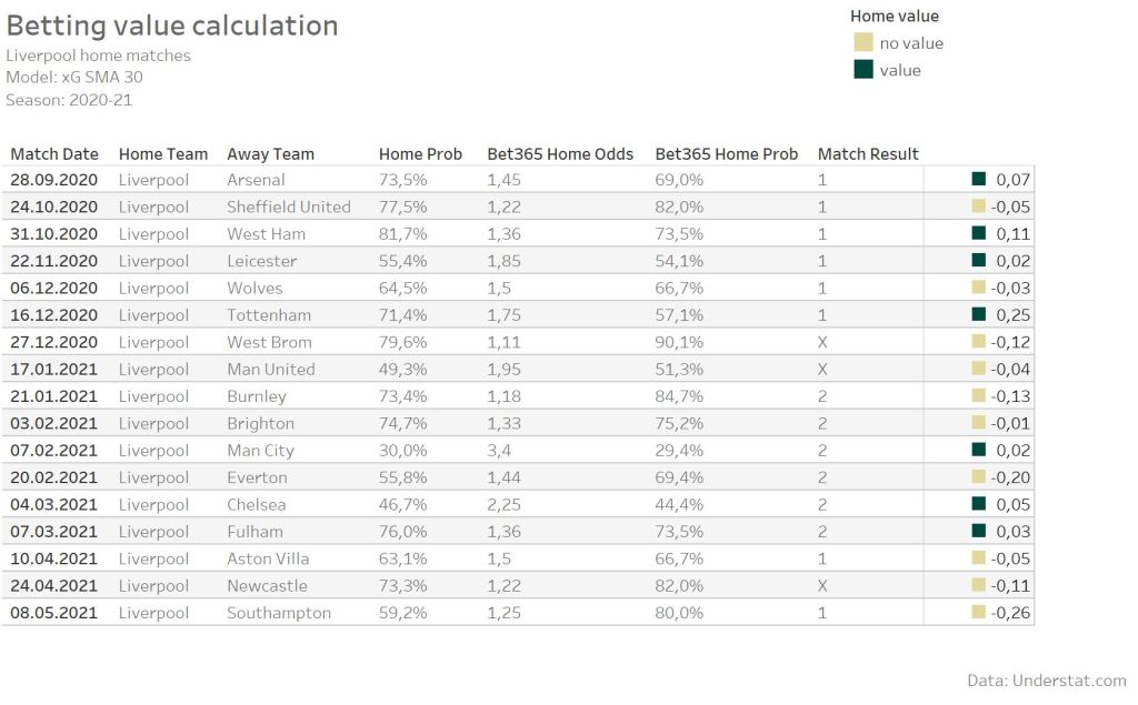
As an example we can take a look at the home matches from Liverpool again. At the beginning of the season the xG SMA 30 model indicates a value, when betting on home win for some single matches. But overall it’s more rare having value on home wins of Liverpool.
For the simulation I always selected just one bet per match, even if a model indicates e.g. the home market and the draw market as value bets. In such cases the market with the higher value was selected. As the Brier score already indicated, a profit could not be expected. While using always 1 unit per bet, the simulation results in a lose between around 800 and 300 units. More interesting is the comparison between the xG and goal models. The xG models definitely performed better. 8 of the Top 10 models use xG data. The 2 models with the biggest lose are based on goals data. Surprisingly the models using more matches for the feature calculation and with the lower Brier score did not perform the best. The models using 5, 10 and 15 matches show the best profit.
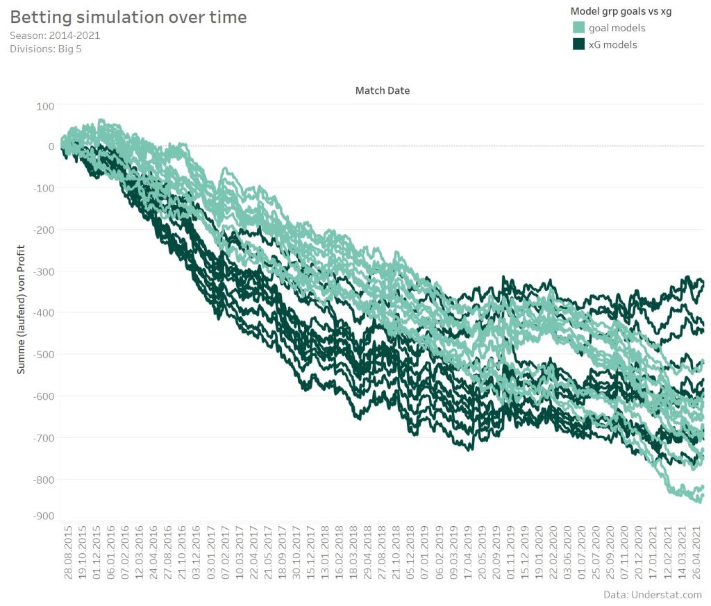
Looking at the simulation over time also reveals something interresting. At the beginning the xG model performed worse than the goal models. With beginning of the season 2017/18 this changed and the xG models followed more a lateral trend. Single models even showed a positiv profit, when just looking at this period. In comparison the goal models just continued the downward trend.
Conclusions
One can still argue about xG values for a single game or individual shots, and such discussions have their justification, of course. But what one cannot argue about is the additional information such a statistic or model provides us. It fills a gap between goals and shot and provides.
- xG data have higher predictive power than goals alone. As shown, even a simple model benefits when goals are replaced by xG. The Poisson model still did not improve enough to beat the market, but the improvement is clearly evident.
- Weighting the latest matches more than older matches is a known model improvement, which was already used in older papers. Surprisingly the influence of such a model adaption seems not as big as expected. Adding more data and information – in this case the xG data – has a higher influence on the accuracy.
- One cannot make a conclusion from the Brier score of a model to the profit. The 3 models with the best profit were not even in the top 10 of the Brier score ranking. How this difference comes about, I can not explain and would have to be further explored.
If you have further questions, feel free to leave a comment or contact me @Mo_Nbg.
References:
[1] Mike J. Maher. Modelling association football scores. Statistica Neerlandica, 36(3):109–118, 1982
[2] Mark J. Dixon and Stuart G. Coles. Modeling association football scores and inefficiencies in the football betting market. Applied Statistics, 46:265–280, 1997.
[3] Dominic Cortis, Inflating or deflating the chance of a draw in soccer, https://www.pinnacle.com/en/betting-articles/Soccer/inflating-or-deflating-the-chance-of-a-draw-in-soccer/
[4] Anthony C. Constantinou and Norman E. Fenton, Solving the problem of inadequate scoring rules for assessing probabilistic football forecast models, http://constantinou.info/downloads/papers/solvingtheproblem.pdf

10 Replies to “The predictive power of xG – Predicting football matches with Expected Goals”