A data journey – market values (part 3)

In the 3rd part of this series, I take a look at the – from my point of view – most important part about my market value data journey: Does the team market value holds some predictive power? If so, I could use it as another feature for my predictive models.

Market value superiority

In a past series I tested two models, which just used the goal superiority and the points per game features to predict the result of a football match. But this time I will use the market value. Therefor we need to define the market value superiority, which is basically just the difference between the home and the away team.

[Market value superiority] = ([home team market value] – [away team market]) / 1000000

If the home team got a higher market value as the away team, the market value superiority match rating is positive. If the away team has a higher market value, it’s negative. As I need some bigger clusters to group matches with a similar market value, I divide the difference by 1 mill. So we get clusters of 1 mill. The match ratings are normal distributed with some big tails. This is caused by the huge market value differences in football, what we could already determine in the last part of this series.

For the prediction I even switched to 10 mill clusters to increase the number of matches per cluster. By doing this, a match between Team A with a market value of 241.000.000€ and Team B with a market value of 249.000.000€ will get a match rating of 0 instead of -8 and the teams are considered as equal.

Correlation test

The next steps are basically the same like in my older series. There I explained some things in more detail. So if you e.g. don’t know, what a correlation test tells you, you should start with these posts.

The data for the correlation test and the regression models can be extracted with following SQL statement:

GitHub – Market value superiority query

As a prerequisite, you should have followed the 1st post of these series.

The last months I just used Python. So it’s a good moment to restart my R-Studio. Loading the data is easily done with the Exasol R library. I already have written,  the market value superiority distribution got very long tails. So very high and very low match rating clusters have less matches. The percentages spread very widely because of the law of small numbers. 

To balance these long tails with outliers, I used 3 different sets for this test. The first set contains all match ratings. The second set contains all match ratings from -50 to 50 and -40 to 40 for the third.

cor(train_data$GS_MATCH_RATING,train_data$PERC_HOME_WIN)
cor(train_data$GS_MATCH_RATING,train_data$PERC_DRAW)
cor(train_data$GS_MATCH_RATING,train_data$PERC_AWAY_WIN)

The market value superiority shows a really strong linear relation to the home win and away win percentage. Cutting the long tails even increases this relation. The draw percentage does not have a linear relation. But that’s not surprising. Draws normally have a polynomial relation.

Regression model

As good as the correlation test looks, you have to keep in mind, that the correlation factor does not tells something  about the predictive power of a possible predictive feature. It just indicates a linear relation, which is a good sign, that it holds some predictive value.

Nevertheless, it would be interesting to test a betting strategy just based on the market value. Therefor I created three different linear regression models.

#linear regression
regr_home = lm(PERC_HOME_WIN ~ MARKET_VALUE_SUPERIORITY, data=train_data)
regr_draw = lm(PERC_DRAW ~ MARKET_VALUE_SUPERIORITY, data=train_data)
regr_away = lm(PERC_AWAY_WIN ~ MARKET_VALUE_SUPERIORITY, data=train_data)

The linear regression model looks really good for home and away wins. Of course, otherwise the correlation test would have been worse. But for the draw model, a polynomial regression model is needed as the data points are not distributed linear.

#polynomial regression
poly_regr_home = lm(PERC_HOME_WIN ~ poly(MARKET_VALUE_SUPERIORITY,2), data=train_data)
poly_regr_draw = lm(PERC_DRAW ~ poly(MARKET_VALUE_SUPERIORITY,2), data=train_data)
poly_regr_away = lm(PERC_AWAY_WIN ~ poly(MARKET_VALUE_SUPERIORITY,2), data=train_data)

Plotting both models for the home win, draw and away win percentage shows exactly this. The lines for the linear and polynomial model for home win and away win percentage look nearly the same. The curved line for the draw percentage suites the data point distribution much better.

These models can now be used to predict the outcome for matches with a specific market value superiority ratings. In my example I used all seasons except the current one to create the regression models. The season 2018/19 was than used to test the predictive power. But as expected, the market value just contains to less information to have a competitive predictive power and gain a profit over long term.

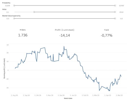
I tried several different combinations: Just betting on relative even games based on the market value,  don’t bet extrem long odds, just take bets which indicate a higher value. Nothing showed profitability. But that’s ok. I did not expect to find the holy grale, when getting all this market value data. I just wanted to get another feature with some predictive value, which can be used to extend and hopefully improve my existing model.

The complete R script for this post can be found at GitHub:

GitHub: Market value superiority R regression model

 

If you have further questions, feel free to leave a comment or contact me @Mo_Nbg.